Modules

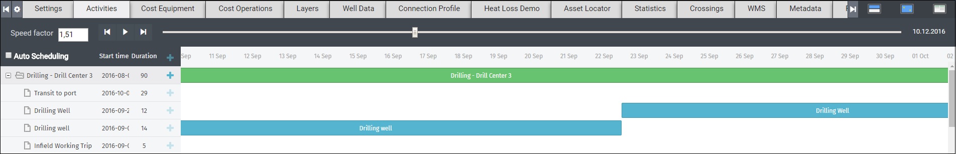
Field Activity Planner provides various functions called Modules that are displayed in seperate tabs on the lower part of the screen as shown below. These are modules for cost calculation, installation/operations planning, connection profiles, Layers, Well Data and much more. Note! The Settings tab will always be shown to the left.

Hide/Show Modules

If you do not use all the modules you can decide, which modules to display on screen, by clicking on the Cog wheel icon next to the Settings tab.

This will display the following dialog:

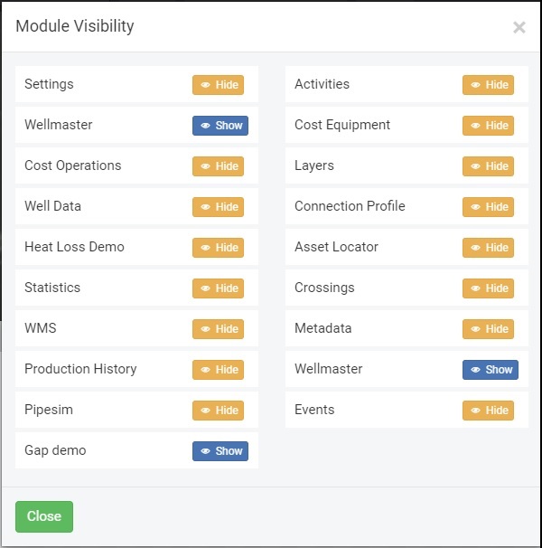
All available modules for your account will be displayed here. Then simply click Hide to disable the ones you do not need displayed. To enable them again, simply press Show.

Asset Locator

With larger field layouts with many assets, and when you are not using condensed mode e.g. vertical/horizontal scale set at 0.1 it can be hard to locate a specific asset or connection without zooming in/out and/or panning around.

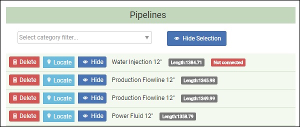
The "Asset Locator" module is now available as a separate tab that will display all your structures, pipelines and umbilicals in a column list view.

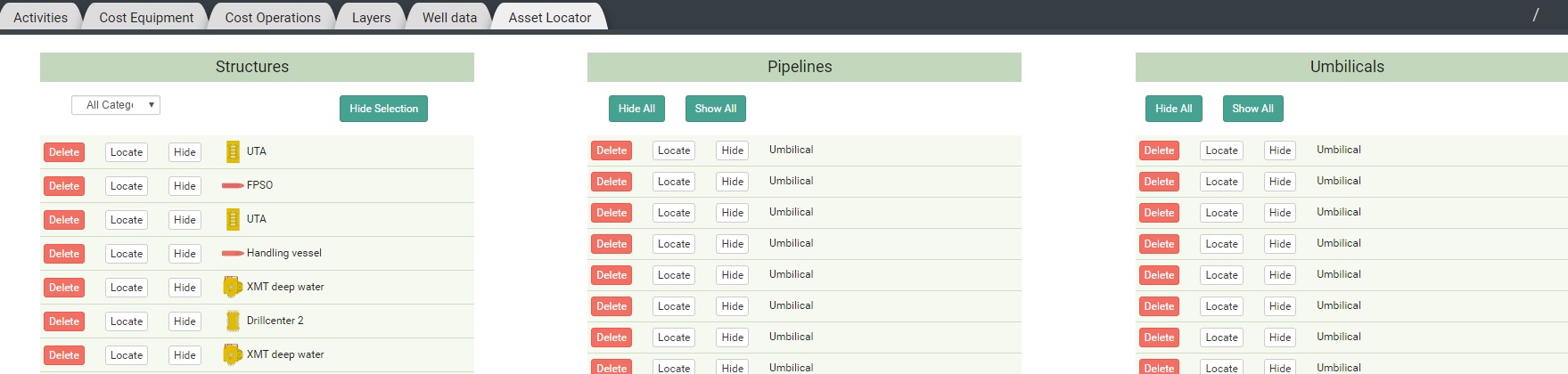
Now you can use that tab and easily locate any asset listed and the stage display will be updated to that specific asset location. You can also "Delete" and Show/Hide" your selection.

Category Selection

You can quickly select a structure category to narrow down your asset selection. Simply select the desired category by using the selection drop down list as shown here:

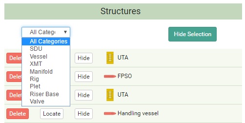
Then select your category e.g. "Manifold" and only the manifolds will be shown in the column list. You can also press the "Hide Selection" button that will then hide the entire category. To display it again, simply press the same button that now shows "Show Selection".

Locator commands

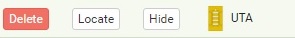
For each asset shown under the Asset Locator tab you have the following available commands; Delete, Locate, and Hide

Delete - Pressing this button for an individual asset will prompt you if you want to delete that specific asset. If you confirm this then the asset will be deleted from the project.

Locate - Pressing this button for an individual asset will then redraw the stage display to be updated to that specific asset location.

Hide - Pressing this button for an individual asset will hide the asset from the stage. Press Show to unhide it .

The asset locator also displays the port location of vessels and rigs that are docked in a port.

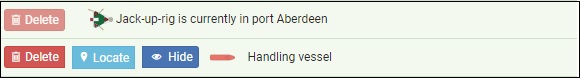
For connections you will also see the length of each connection displayed in meters. And also connections that are not connected to any assets are quickly identified by the red warning indicator as shown below.

Export

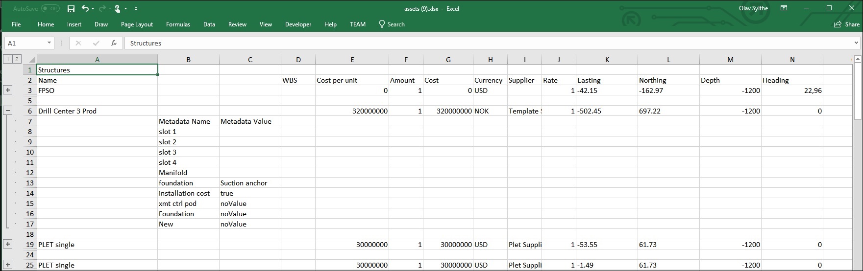
Use the Export button to export out an equipment/bill of material list directly from the Asset Locator module. Only the selected Categories will be exported out in MS Excel format. See the screenshot below for an overview of the various columns that will be exported.

Crossing Detection Module

Identifying crossings of pipes etc. during field design is crucial. The "Crossings Module" will allow the user to quickly locate and highlight any crossings in the field layout. Crossings are costly and this module will allow the user to keep track of the location and number of crossings in the field while also quickly navigating between crossings when working and collaborating on field designs.

To detect all the crossing within the field, select the "Crossings" tab. To generate a list of all the crossing intersections within the field, click the “Detect Crossings,” button. This will then list all connections involved in crossings as shown below:

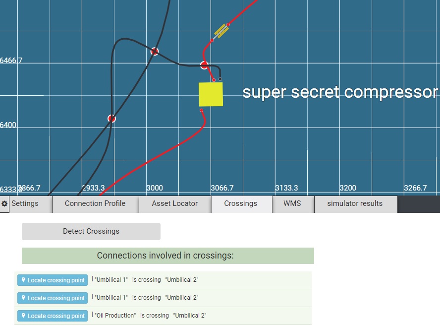
If you have multiple crossings in various locations, simply click on the "Locate crossing point" button to reorient the 2D or 3D stage view to that specific crossing point.

Layer Module

The Layer module allows you to add 2D imagery such as for example shelf and/or seismic maps as a backdrop in the 2D view or 3D view for the Field Layout editor. You can also add multiple background images in (JPEG/PNG/GIF) format. You can also add 3D Surface layers such as Bathymetry/Survey data and/or Reservoir data here.

Bathymetry/Survey data

From version 3.1, you will now add Bathymetry as a layer. Previously, you would load this in project settings and that would automatically define the sea bed level. With version 3.1 the Bathymetry support is moved into the “Layer” module where you load it as a 3D Surface instead. Having the Bathymetry as a layer allows us to now let you load multiple Bathymetry files as individual layers to allow support for fields with multiple surveys and bathymetry data for a single project. FieldAP will then height- or depth-sample if you will each Bathymetry layer individually, and where there is no Bathymetry data the default “Sea Level” value from the Project settings will be used.

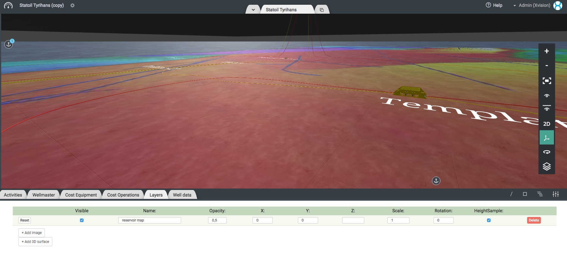
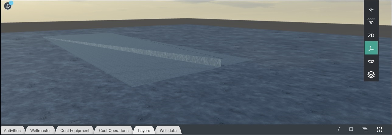
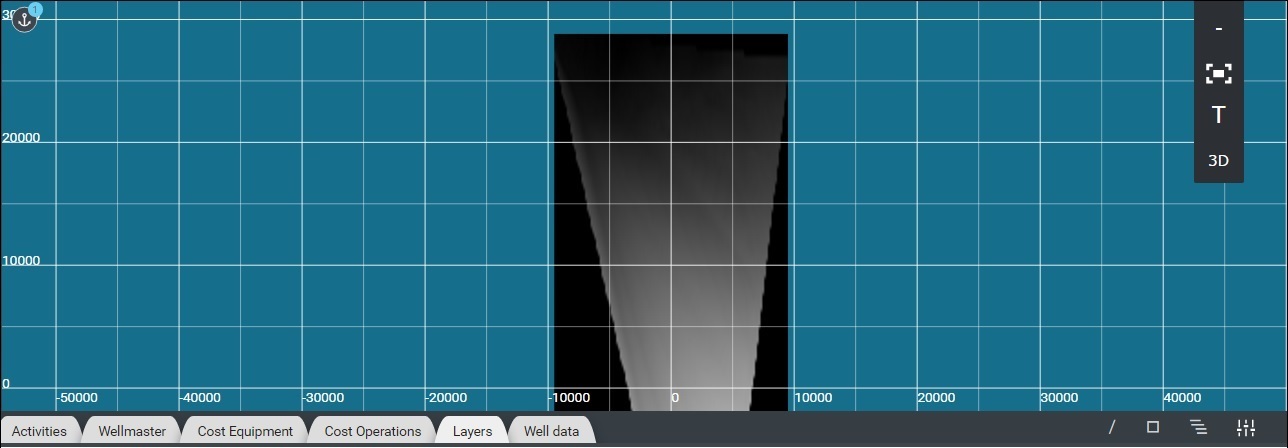
Layer showing in 2D mode:

Layer showing in 3D mode:

Create Layer

To add a new image Layer in the background simply click on the "+Add image" button. This will display a dialog that will allow you to select a file and add it as a new layer with a descriptive name of your choosing.

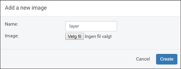
Multiple layers can be added by clicking the "+Add image" button again.

Layer Attributes

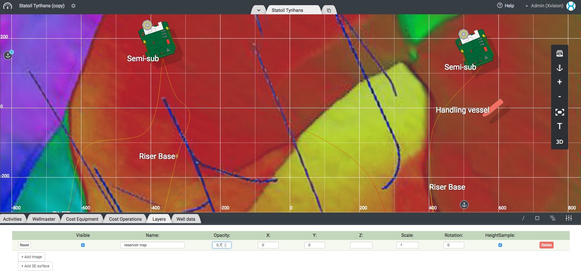
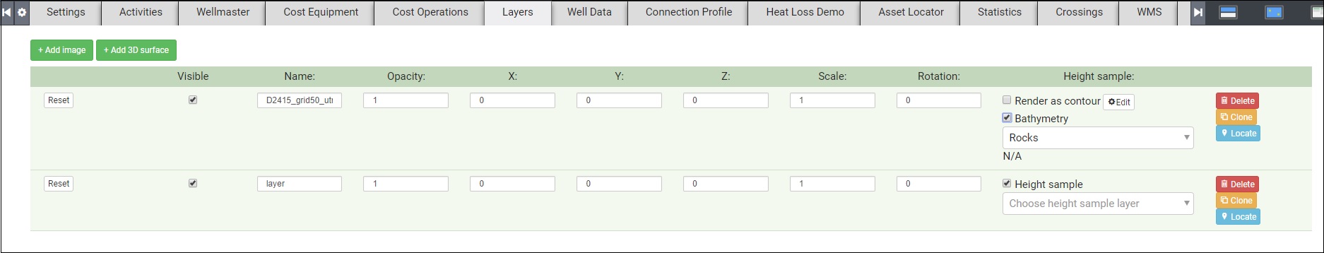
You can manipulate the following layer attributes directly in the "Layer Module" tab; "Visible", "Name", "Opacity", "X" position, "Y" Position, "Z" Position, "Scale", "Rotation" and various "HeightSample" options.

• Visible - Displays the layer if checked. Allows you toggle layers on/off.

• Name - The descriptive name you assigned to it when adding the image. Can be changed at any time.

• Opacity - Allows you to adjust the transparency of the layer by adjusting the value between 1 (Fully Visible) and 0(Invisible).

• X - Change the X position (horizontal) of the image placement which is inserted to a 0 origin position by default. Negative values will shift the image left. Positive values will shift the image right.

• Y - Change the Y position (vertical) of the image placement which is inserted to a 0 origin position by default. Negative values will shift the image up. Positive values will shift the image down.

• Z - Change the Z position (depth) of the image placement which is inserted to a 0 origin position by default.

• Scale - Allows you to adjust the scale of the layer by adjusting the value up (larger) or downwards (smaller). The default value of 1 is the original size.

• Rotation - Set the rotation of the image in the layer by adjusting the value between 0 and 360 degrees.

HeightSample Options

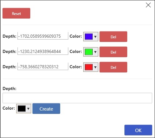
• Render as contour - We have added support for simulating rendering of HCPT (Hydrocarbon Pore Column Thickness) data and represent these as contour plots based on assign the color gradient for the Z value. When loading such a file set “Always negate depth” to “No”. Then select this option. You can then select which 3D layer to height sample the “Contour plot” to. You can change the Z color sample values, by clicking on the Edit button. This will display the dialog for setting the Z depth color association for rendering as shown below.

• Bathymetry - Select this option if the 3D surface data loaded is Bathymetry/Survey data to be used in the project.

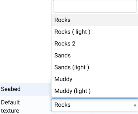
• New Bathymetry Textures - You can change between different textures to be used in 3D view to better illustrate the seabed type e.g. sand or rocks. We have improved the texture quality and added new texture types that can be applied to the Seabed under “Settings” as shown in the illustration below. You set your selection using the drop-down list as shown here:

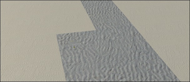
As with Bathymetry described above you can also use these new textures for the default seabed rendering in 3D view. See the “Settings” options for more information. These new texture settings allows you now to have different textures on both the seabed and the bathymetry as shown in the illustration below using:

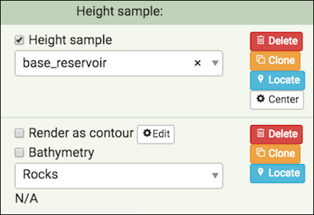
• Height sample - This allows you to select a 3D surface layer from a drop down list of loaded 3D surface layers to height sample a 2D image or a Contour plot onto. This can be applied to the bathymetry under the “Layer” module as shown below:

Reset Values

You can reset all values to default at any time by pressing the "Reset" button.

Delete Layer

You can delete a layer by clicking the "Delete" button. Note! This operation cannot be undone.

Clone Layer

You can clone a layer by clicking the "Clone" button.

Locate Layer

You can locate a layer by clicking the "Locate" button.

Add 3D surface

To add a new 3D surface layer e.g. Bathymetry/Survey or Reservoir data in the background, simply click on the "+Add 3D surface" button. This will display a dialog that will allow you to select a file and add it as a new 3D surface layer. The default name will be set to the filename, but you can change it in the Name field with a descriptive name of your choosing.

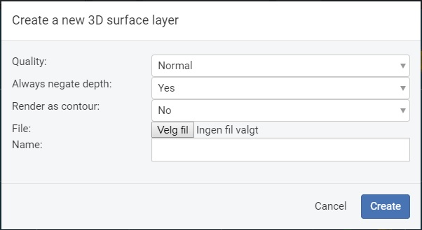
Quality - Allows you to select the conversion quality on the 3D surface file you wish to upload. You can choose between; Low, Normal, High, and Extreme. This defines the resolution of the 3D mesh created. The default selection is Normal, which is a good tradeoff between speed and resolution.

Since this is a browser based solution and given the size and dimensions of the bathymetry files we resample the bathymetry data on conversion on the server side so it can be sampled real time in the browser. So based on the quality setting we map the bathymetry to a texture which is then also resized to best fit the aspect ratio of the bathymetry area. The quality settings are resampled as follows:

Extreme:    512x512 pixels
High:       256x256 pixels
Normal:     128x128  pixels
Low:        64x62 pixels

To examplify for a 4 x 2 km bathymetry file with the "Normal" setting and with aspect ratio applied the conversion will use a 256 x 64 setting making 1 pixel equal 4000/256 m = 15,6 meters

For a 5 x 5 km bathymetry file with "High" setting the resolution will be 5000/256 = 19,5m and for "Extreme" 5000/512= 9,7 m per pixel

Please note! You can upload multiple bathymety files with varying resolution in the same project so you can have e.g. a more detailed DEM for areas around a pipeline.

Always negate depth - This option allows you to load land based elevation models e.g. DEMs that have positive height or Z values. Set this to "No" and you will display the 3D surface model above sea level.

File - This will display a file dialog for selection of the 3D surface file you wish to add as a layer.

Name - This field will allow you to change the name of the 3D surface file that will be converted to a more meaningful layer name. By default this will be populated by the file name selected.

Create - Then click on Create to have the file automatically converted and added to your project. Click Cancel - to abort.

The file will then be uploaded and converted and displayed on screen when complete and the new 3D surface layer will be shown in the layer module.

The 3D surface layer will also be visible when you switch to 2D View mode as a depth map is automatically created from the 3D surface for this purpose to assist you with you field design activities. See illustration below.

The 3D surface layer attributes are the same as for the Layer Attributes.

Hillshade Lighting Effect for Bathymetry data

New in this version is the simulation of hillshades. A hillshade is a grayscale 3D representation of the surface, with the sun's relative position taken into account for shading the image. Applying hillshade lighting to Bathymetry will create a relief map of the bathymetry or landscape if you will that will provide better detail for deciding your field layout and pipeline routing.

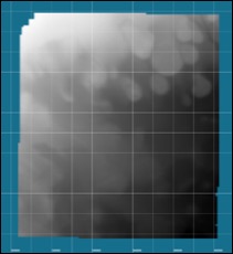
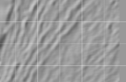
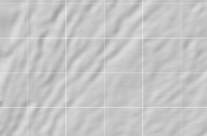
Today uploaded bathymetry into Field Activity Planner will look like the leftmost image in 2D view, which does not yield to much useful detail as the 2D representation is a simple depth map: Applying the real time hillshade effect on the same bathymetry will yield another result that reveals much more detail about the actual topography e.g seabed:

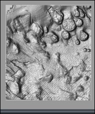
As you can see the relief map of the same bathymetry created in real time is now much more useful with providing geographical detail for especially your pipeline routing design as one example.

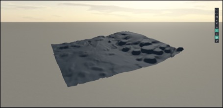
If we switch to 3D view the screenshot below shows the bathymetry only with no hillshade lighting applied.

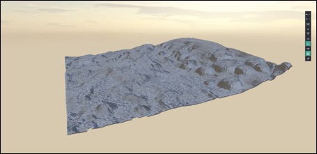
If you apply hillshade lighting, it will look as follows and reveal more detail of the seabed topography.

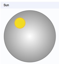
For this new feature to be effective you will need to load new or reupload bathymetry to your project as we compute a “Normal” map when converting the bathymetry data on the backend to achieve this effect. This effect works for both 2D and 3D view and you adjust the sun’s relative position in the “Settings” tab with the “Sun” dial. See the screenshots below where you see two 2D representations of the bathymetry with different Sun position settings. When changing the sun position the hillshade lighting changes in real time so you see immediate results.

3D Reservoir Module

This new reservoir visualization module for Field Activity Planner can help accelerate your field planning and development activities by showing the real reservoir data in 3D with the number of wells required. Additionally, you can also see the real world position of both the top and bottom hole for each individual well along with well trajectories.

By combining information sources such as reservoir, seismic, and real well-data with your visualized field layout in 3D you immediately obtain a better understanding of the complete project.

Enabling Reservoir Mode

To enable the Reservoir mode select the following icon from the 3D View toolbar.

When the Reservoir mode is enabled the seabed will turn translucent to allow you to view layers and/or 3D data that are positioned below the actual seabed level e.g. the reservoir data sources.

If you add bitmap imagery as layers you can freely position, rotate and scale them as any normal layer above the seabed. You do this in the layer module as described in the Layer Module

With 3D data is loaded in it is placed as an individual layer. But unlike standard bitmap layers you can only manipulate visibility on/off and opacity. This is because the correct scale, position and rotation is embedded in the converted 3D data and is correctly represented in real world scale.

Typical data that can be displayed beneath the seabed is for example:

Reservoir maps
Well placing maps
Geological formations
3D scan of reservoirs
3D well trajectories

Well Data Module

The Well data module allows you to directly import well trajectory data as ".txt" files directly into Field Activity Planner where they will be displayed in 3D if Reservoir mode is enabled.

Import well data

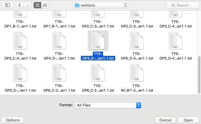
To import a well just press the Import well button and select the trajectory text file for the well you want to display. You can select multiple files to load several wells at once.

This will display a dialog for selecting the well data text files to load.

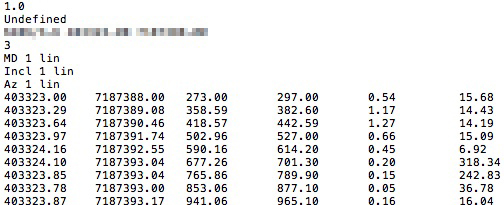
At the moment we support some of the most common well formats for well trajectory data. This will typically look like the following format as shown here:

If the well format is not recognized, an import helper dialog will be displayed:

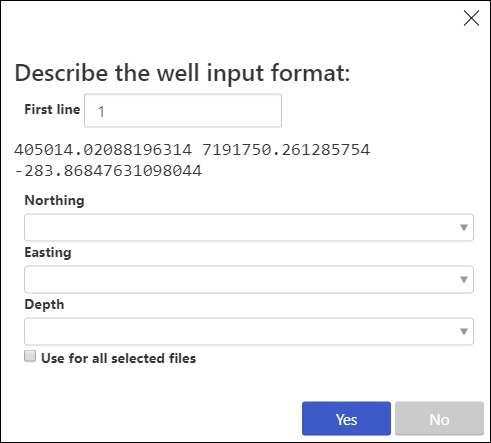
This will allow you to describe the well format file by using the following parameters.

First line - This number specfies which line number the x,y,z data should be read from e.g. this allows you to skip well data headers. Typically the first 3-7 lines of text.

Northing - This drop down list will display the first 3 columns of values read from the file as Col 0-2. Assign the appropriate column value as the Northing coordinate value.

Easting - This drop down list will display the first 3 columns of values read from the file as Col 0-2. Assign the appropriate column value as the Easting coordinate value.

Depth - This drop down list will display the first 3 columns of values read from the file as Col 0-2. Assign the appropriate column value as the Depth value.

Use for all selected files - Check this option if you are importing multiple well files at once and they all have the same format.

The Well Data Module is now updated the possibility to turn on the display of the imported or renamed name of the well next to its location as well as displaying the length of each loaded well in meters in the “Length” column. When the well(s) trajectories are loaded you will see them listed as below:

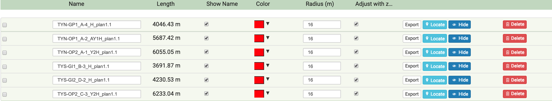
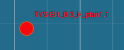
To display the Well Name just toggle the checkbox “Show Name”, and the well name will appear next to the well as shown below. You can also freely position the text label.

To export a loaded Well profile, simply click on the “Export” button and a text file with the well profile in X, Y, Z coordinates will be downloaded to your computer.

None selected - This section handles operations on multiple wells. Tick the checkbox to select all wells automatically. Uncheck the box to unselect them. You can also select individual wells from the list below into a selection to perform operations on. The functions you can perform on the selection are the same as on an individual well entry. The commands are described below.

Name - Edit the field to give the well an identifiable name if you you do not want to use the file name. The check box to the left is if you want to add it to a mutiple selction set.

Color - Select the color for the well display by using the color picker.

Radius - Change the Radius value to control the size of the well display in 2D and 3D stage view.

Adjust with zoom - Select this option if you want the well render size to be adjusted when you zoom in or out.

Export - This will export the selected well path out to an x,y,z file. Use Export selection to export all selected wells.

Locate - Press this button to locate the well in 2D or 3D view.

Hide/Show - This button will hide or show the selected well. Use Show/Hide selection to perform the operation on multiple wells.

Delete - Press this button to delete the selected well. Use Delete selection to perform the operation on multiple wells.

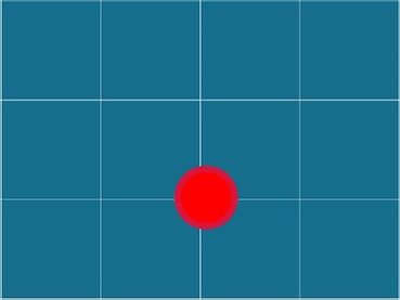
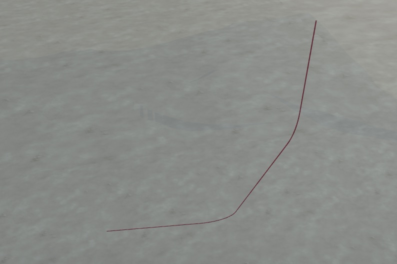
The well will be placed in 3D according to the coordinates from the well data text file. If you switch to 2D View the loaded wells are visualized as red circle(s) with a color inside (the color is selectable).

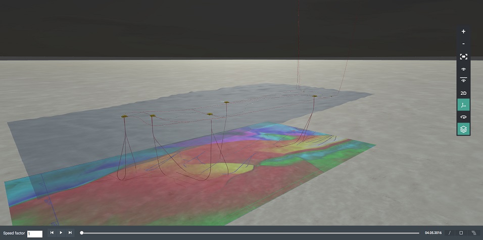
In 3D mode you will see the entire trajectory of the well (reservoir mode enabled).

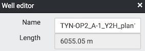
Well Editor Module

In this version you will also find the first iteration of the “Well Editor” that will in the future allow you to manipulate top hole, and downhole locations and other well attributes. At the moment it will only display the Well Name and Length for the selected well as shown here:

Connection Profile

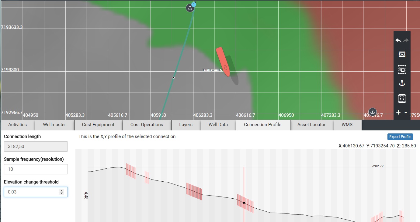
This module enables a 2D profile or side-view of how a selected connection follows/samples the seabed/bathymetry and allows you to get a better understanding of the elevation changes for the selected connection.

When a connection is selected you can move your mouse sideways to move the indicator along the connection profile display. It will then display the actual depth in meters at that specific point. You will also see a circular visual indicator move along the connection in 2D or 3D stage view at the same time to indicate the exact position for the sample readout. You will also see the current X, Y, Z coordinate values displayed on screen as you move the mouse.

The legend displays the minimum and maximum depth of the selected connection, and to the left you will find the selected connection length in meters. You also have two input fields namely Sample frequency (resolution), and Elevation change threshold.

Sample frequency (resolution)

The sample frequency allows you set the distance in meters between each depth sample reading on the connection.

Elevation change threshold

Elevation change sets the threshold value in meters on how much the connection elevation can change between each sample point. If the elevation exceeds this value, the display will mark the point with a red vertical bar to pinpoint the location.

Export Profile

You can at any time click the Export Profile button, and a text file in x,y,z format will be saved with the x,y,z coordinates for the entire selected connection profile. The number of points in the file is determined by the value in the Sample frequency field that is defined in meters. If you enter a value of 10 here the x,y,z file will save out the coordinates every 10 meters on the selected connection.

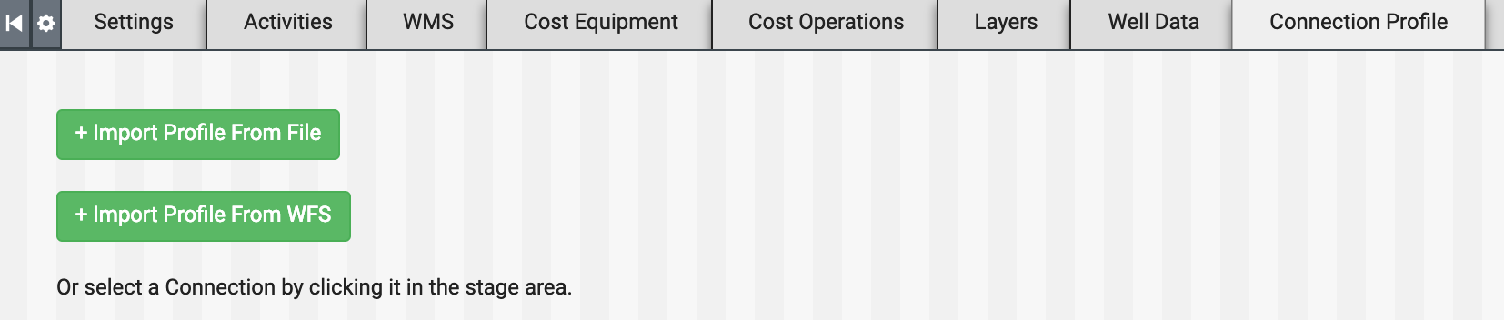
Import Profile

If no connection is selected when this module is activated you will be presented with two options to import profiles; +Import Profile From File and +Import Profile From WFS.

+Import Profile From File This option allows you to import connection profiles in x,y,z format from other engineering SW/tools into Field Activity Planner for more accurate display of connections. In the dialog, select if you want the Z value to be sampled to the bathymetry data or not. This option allows for the import of e.g. externally calculated riser profiles from SW such as OrcaFlex if you leave the option “The connection follows the seabed” unchecked.

Note! After the connection is imported, you will need to manually connect it to assets yourself. If you are unsure of the location of where the connection was imported to, use the Asset Locator module.

+Import Profile From WFS

This feature supports direct import from WFS (read: Web Feature Service) mapping servers/services such as e.g. ArcGIS. Before FieldAP only displayed WMS as an informational layer or visual backdrop if you will. Now you can directly import e.g. existing pipeline data as new connections in FieldAP. This is available in the “Connection Profile” module by selecting the “+Import profile from WFS” button.

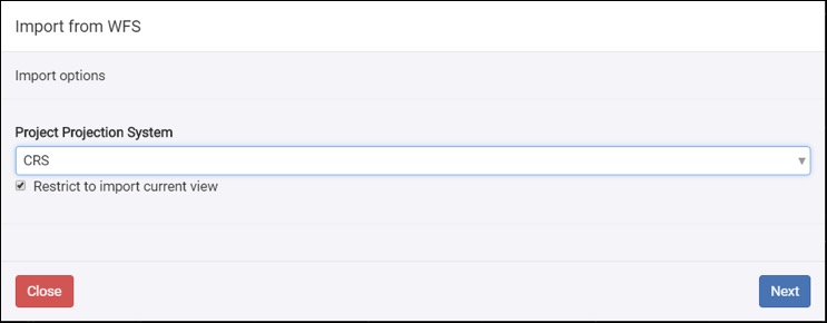
Pressing the button will bring up the following dialog box where you select project projection system to be used from the drop-down list. If you want to restrict the import to the current on screen view you select the “Restrict to import current view” check box as shown below.

Then select “Next” and the following dialog will be shown:

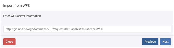
Here you input the WFS server address that you will query for data. This example retrieves data from the Norwegian Petroleum Directorate free mapping service, which you can read about here https://www.npd.no/en/facts/factpages/ Then press “Next“ to continue the process.

This brings up a dialog that list all the available described data layers from WFS query (read: GetFeature) as shown below:

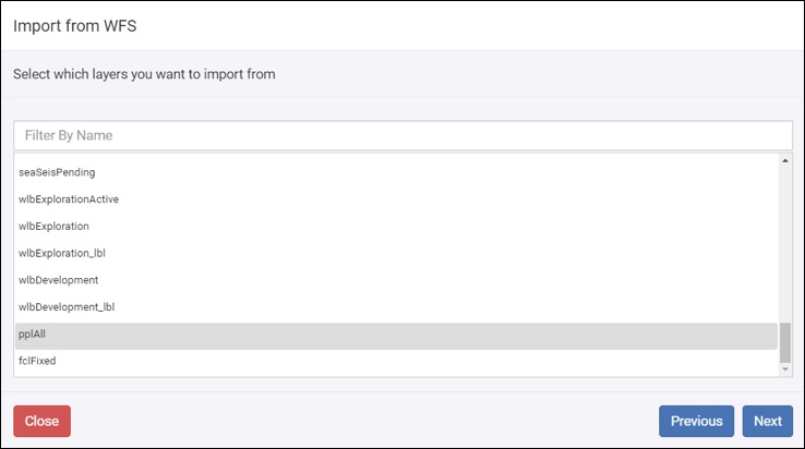
In this sample we selected “pplAll” e.g. all pipelines, and that will present a dialog listing all the available pipelines from this layer:

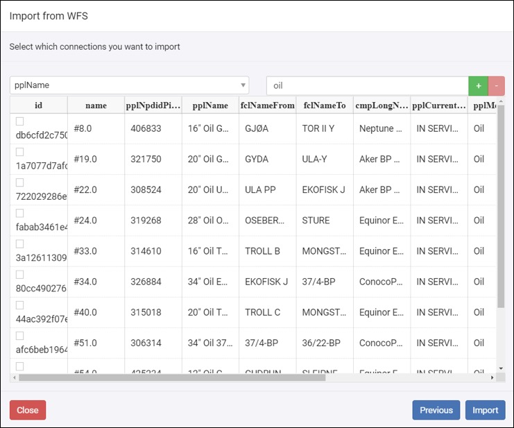
You also have filtering options for “Attribute” and “Value”. For this sample we set “pplName” to “troll”. You can use the “+” and “-“ buttons shown to add or delete filters.

Then press the “Import” button to start the import from the WFS server. A message when the import process is complete will appear. Note! The imported connection might not show up on the screen as that depends on the current field location. The easiest is to select the “Asset Locator” module and use the “Locate” function to be taken to the imported pipeline as shown below.

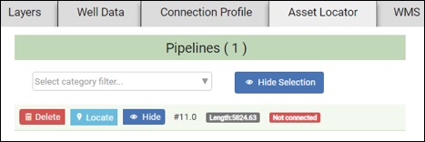
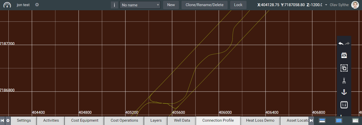
Press “Locate” to jump to the imported pipeline as shown here:

Support for GeoJSON files

The connection profile module is now supporting import of connections or pipelines if you will in both GeoJSON file format. Many WMS (mapping) servers like ArcGIS allows you to extract/export pipelines in GeoJSON format if you store your facility data there, or from CAD software you can typically save or export these as “SHP” files. To import these type of data formats into FieldAP, select th“Connection Profile” module. Then click on the “+Import Profile” button and confirm if you want the imported data’s Z values to follow the existing seabed/bathymetry or retain the original Z values in the file. Then select the file and press “Open”.

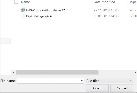
And the file will be imported into FieldAP and displayed as shown below:

Support for SHP files import in Connection Profile module

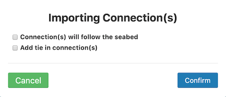
The connection profile module is now supporting import of connections or pipelines if you will in Shape (SHP) file format. Most CAD software will allow you to save or export your pipelines as “SHP” files. To import these type of data formats into FieldAP, select the “Connection Profile” module. Then click on the “+Import Profile from File” button and confirm if you want the imported data’s Z values to follow the existing seabed/bathymetry or retain the original Z values in the file. You can also select “Add tie-in connections” for the imported SHP files. This feature adds one additional point at both ends of the imported .SHP file. E.g. there is a long distance between the first and second point in the pipeline and you want to adjust the begiining of the pipe to tie in to a plem or similar, you have to add a new point to create the last bend. So this feature creates these "tie-in" points automaticly.

Pressing “Confirm” will then display a file selection dialog.

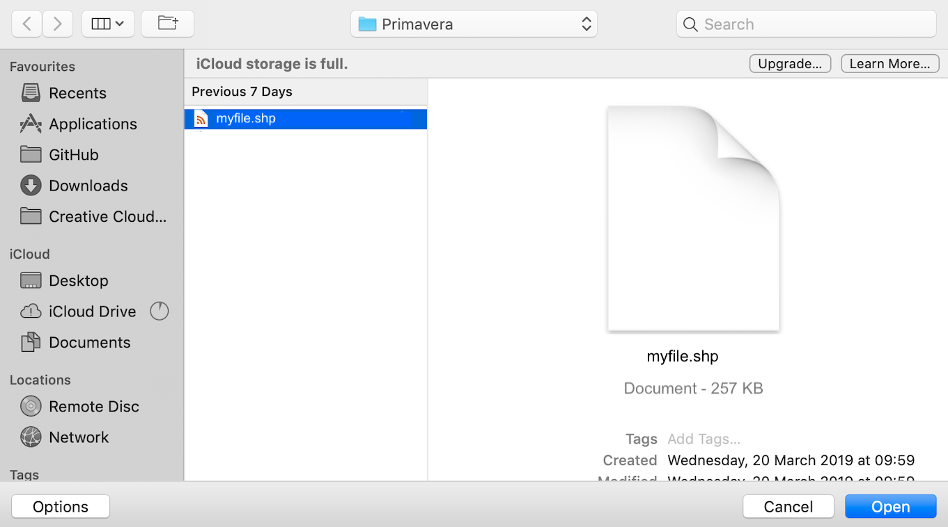
Select the SHP file you want and press “Open” and the file will be imported into FieldAP and displayed as show below:

Depending on the coordinates of the imported connection you might need to use the “Asset Locator” module “Locate” function to quickly find the imported connection. We also support GeoJSON files for import with this feature.

WMS Module

The use of geography data is becoming more and more important for oil and gas operators and service providers to make informed decisions. This can be in terms of locating and extracting new resources, better field design and planning, information retrieval and offers deeper insight into relationships and patterns as part of everyday operations. You can add a map layer to Field Activity Planner using the WMS (Web Mapping Service) Module.

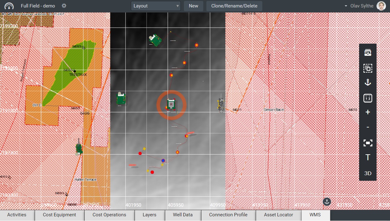
As an example, if you are working on project on the Norwegian continental shelf you can now access the Norwegian Petroleum Directory open map service and visualize information such as wellbores, surveys, fields and discoveries, production licenses, agreement-based areas, permanent facilities and more as part of your layout to facilitate more effective discussions for e.g. equipment and piping scenarios. You can also directly connect your on-premise GIS software e.g. ArcGIS servers or similar.

Setting up WMS server

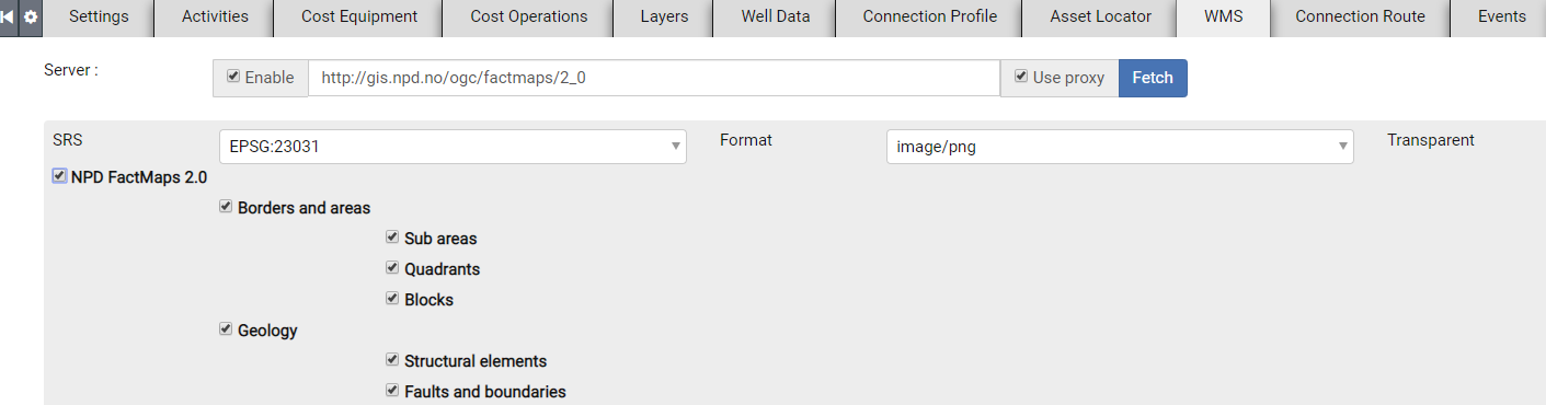
To add a map layer to FieldAP simply select the WMS module tab and define the required WMS server fields.

Enter the WMS service URL in the Server field, and check the enable checkbox. Depending on your network settings, or if you want to access a non HTTPS WMS you will have to check the use proxy selection. Then click on Fetch, and FieldAP will call the GetCapabilities function.

As an example this is the URL for the NPD map service

http://npdwms.npd.no/npdwmsmap_WGS84.asp

WMS GetCapabilities

After you have pressed Fetch the WMS module will display the various configuration options returned by the WMS GetCapabilities call below the Server field. These you can then configure as you see fit. Please see the WMS map service documentation for more information.